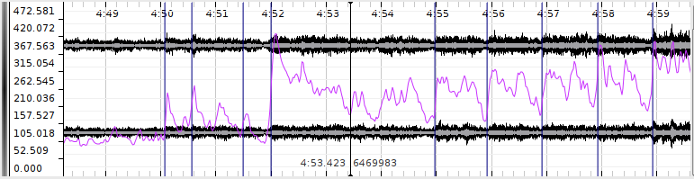
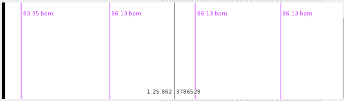
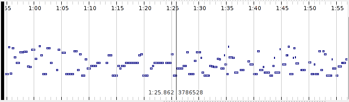
A pane with four layers: waveform in black, time ruler in grey, time values in purple and time instants in blue.
Note: This reference manual is for a version of Sonic Visualiser that is no longer the latest version. Please consult the Sonic Visualiser website for more details.
Sonic Visualiser is an application for viewing and analysing the contents of music audio files. This is a brief reference manual explaining the concepts used in Sonic Visualiser and how to use it. This manual describes Sonic Visualiser version 1.0.
This document is Copyright 2006-2007 Chris Cannam and Queen Mary, University of London. You may modify and redistribute it under the terms of the Creative Commons Attribution-ShareAlike 2.5 License. See http://creativecommons.org/licenses/by-sa/2.5/ for details.
Please report errors and omissions using the Sonic Visualiser bug tracker.
Sonic Visualiser's user interface is structured around panes and layers. A pane is a horizontally scrollable area of window like a drawing canvas; a layer is one of a set of things that can be shown on a pane, such as a waveform, a line graph of measurements, or a subdivision of the horizontal axis into differently coloured segments.
You can stack as many panes above one another vertically as will fit on the screen. The horizontal axis of each pane corresponds to time in audio sample frames, and all of the stacked panes will be aligned to the same sample frame at their centre points.
Each pane can then display any number of layers, which are conceptually stacked on top of one another like layers in a graphics application. So for example, you may have a spectrogram layer "at the back", with measurements, onset positions and notes displayed in separate layers "in front", i.e. drawn over the top of it. There are several different kinds of layer, which differ in the types of data they can represent: instants, curves (time-value plots), and so on.
Layers that are stacked on the same pane will always share the same magnification and alignment on the x (time) axis. However, they do not have to have identical scales on the y axis – although Sonic Visualiser will attempt to align them by default if their scale units match.
 One pane is always the "active" pane, and this one is marked with a
black vertical bar to its left. The front layer on that pane is the
active layer. Any menu operation in Sonic Visualiser that works on a single layer
will always operate on the active layer.
One pane is always the "active" pane, and this one is marked with a
black vertical bar to its left. The front layer on that pane is the
active layer. Any menu operation in Sonic Visualiser that works on a single layer
will always operate on the active layer.
While most of the annotation layer types are interactively editable on the pane itself, layers corresponding directly to audio data (such as waveform and spectrogram layers) are not.
Sonic Visualiser starts with a single visible pane. When you import an audio file, it adds time ruler and waveform layers to that pane, displaying the new audio file.
There are then three menus dedicated to adding new panes and layers to the display, with various kinds of data in them:
You can also add a new layer by importing an existing set of annotation data from a file.
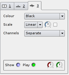
 Each layer, whether editable or not, has a set of adjustable
display properties. These are shown in a corresponding stack to the
right of the pane. To save space, not all of the names of the
properties are shown; you can hold the mouse pointer over a control to
see the name of its property in a tooltip.
Each layer, whether editable or not, has a set of adjustable
display properties. These are shown in a corresponding stack to the
right of the pane. To save space, not all of the names of the
properties are shown; you can hold the mouse pointer over a control to
see the name of its property in a tooltip.
Click on the numbered tab for a layer in this stack to "raise" that layer to the front of the pane and adjust its properties. The available properties for the different layer types are discussed in the sections about those layers, below.
 There is also a tab corresponding to the pane itself, which can
be used to control the way the pane tracks during playback and its
alignment with other panes.
There is also a tab corresponding to the pane itself, which can
be used to control the way the pane tracks during playback and its
alignment with other panes.
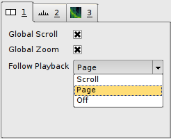
The Global Scroll and Global Zoom settings (both on by default) make the pane follow any horizontal scrolling and zooming that happens in other panes that also have these settings on, so that when you scroll or zoom in one of them, they all scroll or zoom.
The Follow Playback control allows you to choose whether the pane will track playback using a playback cursor, paging when it reaches the edge of the pane (Page); or whether it will scroll along with the playback (Scroll); or neither.
A Sonic Visualiser "session" is a record of almost everything you see in front of you in the Sonic Visualiser window: the current layout of panes, the set of layers on each one, all of the data in each of the editable layers, a reference to the source data (for example the audio file) for non-editable layers like waveforms, the display properties for each layer, and some information about where each layer came from (for example, whether it was generated by a plugin and if so, which plugin and how it was configured.)
You can save the entire session to a .sv session file using File ->
Save Session As... Reloading this file should restore your session
state, provided that the original audio file can also be found. (If
you are passing session files to other Sonic Visualiser users, be sure to make sure
they have the audio data as well, as this is never stored in the
session file.)
Sonic Visualiser provides full multi-level Undo and Redo. Almost all actions that change the session you see in front of you – with the exception of scrolling and zooming – can be undone. This includes adding and removing layers and panes and changing the display properties for a layer, as well as more conventional edits.
Sonic Visualiser has four "tools", which control the way mouse actions interact with the panes. These can be activated using the four tool icons on the toolbar:
With the select tool ![]() active, click and drag
within any pane to select a region.
active, click and drag
within any pane to select a region.
The selection boundaries will snap to the resolution or features present on the active layer. For example, if you drag a selection on a spectrogram layer, the selection's boundaries will be aligned with the spectrogram's FFT window hops; if you drag a selection on a time-instants layer, its boundaries will snap to instants present on the layer; if you drag a selection on a waveform layer, its boundaries will simply snap to audio sample frames.
Pressing Shift as you start dragging a selection will defeat this snap effect, forcing the selection to snap to the nearest audio sample to each pixel boundary.
You can select more than one separate region at a time, by holding Ctrl as you start selecting the second and subsequent regions to add them to the existing selection.
You can also click-drag the left and right edges of a selection to change its extents after it has been made.
A selection within Sonic Visualiser conceptually consists of one or more regions in time. When you select a region in a layer, you are selecting a period of time across all layers; you are not selecting the visible items that happen to fall within that region in that one layer.
This has several consequences:
An advantage of this is that it is very easy to select all the items in one layer that fall between certain items in another layer – make the second layer active, make a selection (which will snap to the item positions on that layer), then make the first layer active again.
Most of Sonic Visualiser's annotation layer types are interactively editable. Layers corresponding directly to audio data (such as waveform and spectrogram layers) are not editable. Sonic Visualiser is not an audio editor.
To move an individual item in a layer, make sure the
edit tool ![]() is active and then click on and drag
the item. If the item is relatively wide on the screen, you may have
to click and drag its left hand edge for the drag to take effect.
is active and then click on and drag
the item. If the item is relatively wide on the screen, you may have
to click and drag its left hand edge for the drag to take effect.
You can also edit the details of an item directly, by double-clicking
on it with either the navigate ![]() or edit
or edit ![]() tool selected. (The advantage
of using the navigate tool is that it removes the risk of
accidentally editing the point while double-clicking on it.)
tool selected. (The advantage
of using the navigate tool is that it removes the risk of
accidentally editing the point while double-clicking on it.)
To move a set of items at once, select the region around them, then switch to the edit tool ![]() and drag the selected
region.
and drag the selected
region.
To delete one or more items, select the region around them, then use Edit -> Delete Selected Items.
Sonic Visualiser allows you to cut and paste between layers of different types, preserving as much information as can be reconciled with the layer types.
 To cut and paste between two layers, select the items in the source
layer, use Edit -> Cut, select the target layer and Edit -> Paste.
The items will be pasted at the same location in time as they were
found in the source layer.
To cut and paste between two layers, select the items in the source
layer, use Edit -> Cut, select the target layer and Edit -> Paste.
The items will be pasted at the same location in time as they were
found in the source layer.
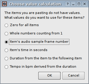
If the target layer is of a type that represents less information than the source – for example if you are pasting to a time instant layer from a time/value curve – then the relevant information (in this case time positions) will be retained, and the rest discarded.
If the target layer represents more information than the source, you will be offered various options for how to make up the values that are not present in the pasted items (as shown to the right).
The waveform layer shows audio data in a traditional waveform peak display.
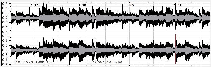
Each pixel on the horizontal axis shows the peak and mean positive and negative values found in samples falling within that pixel's range at the current zoom level. The zoom level can be increased or decreased in multiples of sqrt(2) using the mouse wheel or the Up and Down cursor keys.
The Y axis scale can be adjusted using the Scale display properties:
The Scale properties also provide a display gain control, and a "Normalize Visible Area" switch which will adjust the display gain continuously so as to ensure full scale displacement for the largest value in the visible section of the waveform.
The way the waveform layer handles multiple channels can be adjusted using the Channels display property:
The time ruler layer simply displays a series of labelled time divisions.
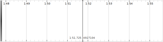
Each new pane has a time ruler layer in it by default, although you can remove or hide it. The time ruler layer is not editable.
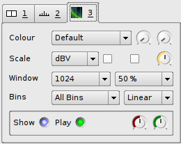
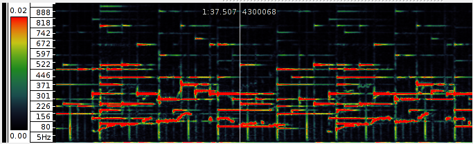
The spectrogram layer shows audio data in the frequency domain, with the Y axis corresponding to frequency and the power (or phase) of each frequency within a given time frame shown by the brightness or colour of the pixels corresponding to that frequency.
There are three types of spectrogram layer available in the Sonic Visualiser menus: "plain", Melodic Range, and Peak Frequency. These differ only in the initial properties the layer is set up with. You can always turn any kind of spectrogram into any other kind by adjusting its properties after it has been created.
The colour scheme used for the spectrogram can be adjusted using the Colour properties (Colour, Threshold, and Colour Rotation). The Colour option allows you to select different colour maps; while most of these are smooth gradients from one colour to another, there are also two colour maps (Banded and Highlight) that employ sudden transitions of colour. These can be useful with the Colour Rotation control to isolate areas with similar levels.
The type of values displayed, and the way the colour scale for the spectrogram is calculated can be adjusted using the Scale display properties:
The spectrogram itself is obtained from the results of a series of fast Fourier transforms of windowed sections of the original audio. The parameters of these transforms can be adjusted using the Window display properties:
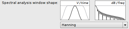 The shape of the window applied to each section of audio data is
not adjustable from the spectrogram properties, but can be adjusted
globally in the application preferences. The
available shaped windows are Hamming, Hanning, Blackman,
Blackman-Harris and Nuttall (cosine-based windows); Gaussian, Parzen,
triangular and un-windowed (rectangular). The Hanning window is the
default and should be appropriate for most purposes.
The shape of the window applied to each section of audio data is
not adjustable from the spectrogram properties, but can be adjusted
globally in the application preferences. The
available shaped windows are Hamming, Hanning, Blackman,
Blackman-Harris and Nuttall (cosine-based windows); Gaussian, Parzen,
triangular and un-windowed (rectangular). The Hanning window is the
default and should be appropriate for most purposes.
The scale used for the Y axis of the spectrogram can be adjusted using the Bins properties.
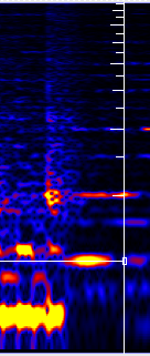 If you switch to the
 ![]() select tool and move the mouse over
the spectrogram, it will show the "harmonic cursor" (see right). This
is a vertical line with tick marks at the frequencies of the second
harmonic, third harmonic and so on of the frequency that the mouse is
currently pointing at. These frequencies are simple multiples of the
fundamental, so they will be equally spaced if the frequency scale is
linear, or will get closer together as they go up if the frequency
scale is logarithmic.
select tool and move the mouse over
the spectrogram, it will show the "harmonic cursor" (see right). This
is a vertical line with tick marks at the frequencies of the second
harmonic, third harmonic and so on of the frequency that the mouse is
currently pointing at. These frequencies are simple multiples of the
fundamental, so they will be equally spaced if the frequency scale is
linear, or will get closer together as they go up if the frequency
scale is logarithmic.
When selecting a region of time in a spectrogram layer, the selection will snap to the spectrogram's processing time frames. Hold the Shift key at the start of selection to defeat this.
The Sonic Visualiser pane and layer menus contain options to add three kinds of spectrogram. These are all the same type of layer, but starting with different display properties.
The plain spectrogram option creates a spectrogram that displays the full frequency range up to half of the audio file's sampling rate, with the vertical Frequency Scale set Linear, with Colour Scale set to dBV, and using the default, fairly gentle green-yellow-red colour scheme.
This is a general overview of the content of the file, in which background noise and overall equalisation trends may be fairly evident but individual musical features are not usually easy to make out.
The melodic range spectrogram aims to make it easier to discern individual musically meaningful features.
It shows by default a frequency range from approx 40Hz to 1.5KHz, covering around 5.5 octaves that most usually contain melodic content. The FFT windows are fairly large for better frequency resolution, and heavily overlapped. The vertical Frequency Scale is logarithmic in frequency, and therefore linear in perceived musical pitch. The Colour Scale is Linear, making noise and lower-level content invisible but making it easier to pick out salient musical events, and a crisp colour scheme is used.
The peak frequency spectrogram is similar to the melodic range spectrogram, but it aims to make it possible to pick out precise frequency content in the material, within certain limitations.
Its Bin Display is set to Frequencies, so that it displays only those bins that are stronger then their neighbouring frequency bins, and for each bin it calculates an estimated frequency using phase unwrapping on the assumption that a stable frequency is present. This frequency is then displayed using a short horizontal line, rather than colouring the whole bin as a block. In good conditions this may produce a fairly accurate estimate of the actual frequency of an individual tone.
The spectrum layer shows a frequency analysis of the audio at a given point in time, like a vertical slice through a spectrogram layer.
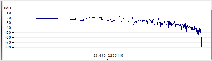
In contrast to almost all of the other layer types, the x axis of a spectrum layer does not measure time. Instead, the spectrum's x axis corresponds to frequency, with lower frequencies to the left and higher to the right. The spectrum animates appropriately to match the movement of time during playback and navigation, instead of scrolling. (In this respect it is closely related to the slice layer, which can display a similar slice through a colour 3D plot.)
The y axis of a spectrum plot shows the value of each frequency bin, corresponding to the colour scale of the spectrogram.
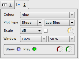 You can adjust the FFT window size
and overlap using the Window properties, just as in the spectrogram;
and you can select the y axis scale (linear or dB), gain and
normalisation using the Scale properties.
You can adjust the FFT window size
and overlap using the Window properties, just as in the spectrogram;
and you can select the y axis scale (linear or dB), gain and
normalisation using the Scale properties.
The type of plot used to show the spectrum can be adjusted using the Plot Type property:
The horizontal extent of each bin depends on the Plot X Scale property, which selects the mapping between frequency and x coordinate for the plot.
The time instants layer shows an editable sequence of points in time (instants), with each point displayed as a vertical bar across the full height of the layer. Each instant may have a label, which will be displayed near the top of the instant.
Instants can be added by clicking with the Draw tool, and edited by
dragging with the edit tool ![]() . You can also
double-click on an instant with the edit or navigate tool
. You can also
double-click on an instant with the edit or navigate tool
![]() to open an edit dialog in which you can change
its label and finely adjust its timing.
to open an edit dialog in which you can change
its label and finely adjust its timing.
When selecting a region of time in a time instants layer, the selection will snap to the nearest instants on the layer (if any). Hold the Shift key at the start of selection to defeat this.
When a time instants layer is active, the fast-forward and rewind buttons can be used to jump the playback position to the nearest instant in either direction.
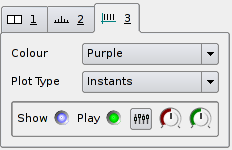
The Plot Type display property can be used to select between Instants display, in which each instant is shown with a single vertical bar, and Segmentation display, in which the regions between instants are coloured in alternating shades.
A time instants layer has a fundamental resolution, as a number of audio sample frames. Instants may only occur at multiples of this resolution, and are displayed using bars of a width corresponding to this resolution. The default resolution is 1 audio sample frame and this cannot currently be changed for any given layer, although layers generated by certain plugin transformations may have different resolutions.
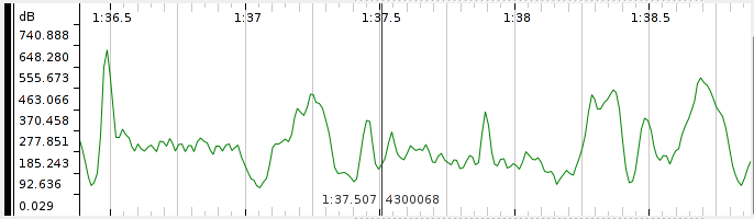
The time values layer shows an editable sequence of points in time, where each point has a value that determines its position on the Y axis. Each point may also have a label.
Points can be added by clicking with the Draw tool, and edited by
dragging with the edit tool ![]() . You can also double-click on a point
with the edit or navigate tool
. You can also double-click on a point
with the edit or navigate tool ![]() to open an edit dialog in which you can
change its label and finely adjust its timing and value.
to open an edit dialog in which you can
change its label and finely adjust its timing and value.
When selecting a region of time in a time values layer, the selection will snap to the nearest instants on the layer (if any). Hold the Shift key at the start of selection to defeat this.
When a time values layer is active, the fast-forward and rewind buttons can be used to jump the playback position to the nearest point in either direction.
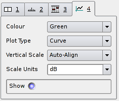
The Plot Type display property can be used to adjust the display of points:
A time values layer may have a unit for the scale on the Y axis. If two layers with the same unit appear on the same pane, they will by default have vertical scales aligned with each other. This behaviour can be adjusted using the Vertical Scale display property.
If Vertical Scale is set to Linear or Log Scale, the scale will cover the range of values (or logs of values) present in the layer; if set to "+/-1", it will cover the range from -1 to +1 and points with values outside that range will be omitted.
If the Vertical Scale for a layer is set to anything other than Auto-Align, then any other layers in the same pane that have the same unit and that have Vertical Scale set to Auto-Align will align themselves to match it.
You can change the scale unit for a layer by selecting from, or editing the value in, the Scale Units property combo-box.
A time values layer has a fundamental resolution, as a number of audio sample frames. Points may only occur at times that are multiples of this resolution, and they may be displayed using boxes of a width corresponding to this resolution. The default resolution is 1 audio sample frame and this cannot currently be changed for any given layer, although layers generated by certain plugin transformations may have different resolutions.
The notes layer shows an editable sequence of notes, where each note has a start time, a duration, and a value that determines its position on the Y axis. Each note may also have a label.
Notes can be added by clicking and dragging with the Draw tool, and
edited by dragging with the edit tool ![]() . You can also double-click on a
note with the edit or navigate tool
. You can also double-click on a
note with the edit or navigate tool ![]() to open an edit dialog in which
you can change its label and finely adjust its timing and value.
to open an edit dialog in which
you can change its label and finely adjust its timing and value.
When selecting a region of time in a notes layer, the selection will snap to the start times of the nearest notes on the layer (if any). Hold the Shift key at the start of selection to defeat this.
A notes layer may have a unit for the scale on the Y axis. If two layers with the same unit appear on the same pane, they will by default have vertical scales aligned with each other. This behaviour can be adjusted using the Vertical Scale display property.
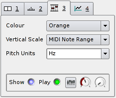
If Vertical Scale is set to Linear or Log Scale, the scale will cover the range of values (or logs of values) present in the layer; if set to "MIDI Note Range", it will cover the range from MIDI notes 0 to 127 and values outside that range will be omitted.
If the Vertical Scale for a layer is set to anything other than Auto-Align, then any other layers in the same pane that have the same unit and that have Vertical Scale set to Auto-Align will align themselves to match it.
You can change the scale unit for a layer by selecting from, or editing the value in, the Pitch Units property combo-box. However, if the scale unit is anything other than "Hz", the layer will assume that the values correspond to MIDI pitch and will convert them to Hz when calculating display and alignment.
A notes layer has a fundamental resolution, as a number of audio sample frames. Notes may only occur at times that are multiples of this resolution. The default resolution is 1 audio sample frame and this cannot currently be changed for any given layer, although layers generated by certain plugin transformations may have different resolutions.
The text layer shows text annotation labels. Each label is fixed to a particular position in time, and appears at a particular height on the layer. The text layer is intended for informal or descriptive annotations that are not attached to other sorts of features (as the other editable layer types allow their points to have labels as well).
Labels can be added by clicking with the Draw tool, and moved by
dragging with the edit tool ![]() . You can also double-click on a label
with the edit or navigate tool
. You can also double-click on a label
with the edit or navigate tool ![]() to open an edit dialog. (You may need
to click at the top-left corner of the text label for an edit to take
effect.)
to open an edit dialog. (You may need
to click at the top-left corner of the text label for an edit to take
effect.)
When selecting a region of time in a text layer, the selection will snap to the nearest label on the layer (if any). Hold the Shift key at the start of selection to defeat this.
The colour 3D plot layer displays a three-dimensional data set in a grid.
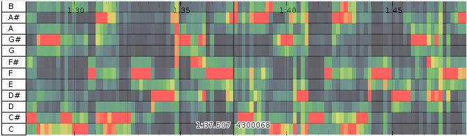
It is used for data sets which have a discrete time axis, a set of bins at each time position, and a value in each bin. (In this respect it resembles the spectrogram, except that the spectrogram also knows about frequencies, window sizes and so on.) The grid x and y coordinates correspond to the time and bin respectively, and each grid square is coloured according to the value in the corresponding bin.
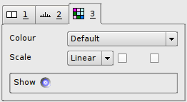 You can change the colour map
used for the value scale using the Colour property; adjust whether the
colour is mapped to a linear or logarithmic scale using the Scale
property; and also choose to normalise the individual columns
of the plot (so that the highest value in each always receives the
brightest available colour) or the visible area of the plot (so that
the highest visible value receives the brightest available colour).
You can change the colour map
used for the value scale using the Colour property; adjust whether the
colour is mapped to a linear or logarithmic scale using the Scale
property; and also choose to normalise the individual columns
of the plot (so that the highest value in each always receives the
brightest available colour) or the visible area of the plot (so that
the highest visible value receives the brightest available colour).
The colour 3D plot layer is not editable. For this reason, you cannot add an empty colour 3D plot layer using the Layer menu, because you would then be unable to do anything with it. These layers only appeard when a transform whose output is appropriate for grid display is applied, or when importing certain types of annotation data.
A slice layer shows an instantaneous graph of the values present along the Y axis of a colour 3D plot layer, at the moment corresponding to the current centre frame. A slice is to a colour 3D plot as a spectrum is to a spectrogram.
If you have a colour 3D plot layer present in Sonic Visualiser, you can add a slice layer for it using the Add Slice of Layer option in the Layer menu.
The Transform menu contains all of the available means of generating new layers with new data in them, using various kinds of binary plugin. If the Transform menu is empty, then you need to get some plugins!
Several types of plugin-based transform are available.
Sonic Visualiser can generate layers using audio analysis and
feature extraction plugins, which may be provided by third party
developers or institutions. The native plugin format is called Vamp
(see http://www.vamp-plugins.org).
Vamp plugins take audio inputs and can generate outputs suitable for
display in any of Sonic Visualiser's standard types of layer.
If you have any Vamp plugins installed, Sonic Visualiser will show
them in the Analysis section of the Transform menu. This section
contains three menus, sorting the available plugin outputs according
to plugin category, plugin name, or the maker of the plugin. Category
information is obtained from an optional .cat file
associated with each plugin library; Vamp plugins that lack categories
will appear in an Unclassified section. (Advanced users may set up
their own category hierarchy by making and installing their own
.cat files: the file format is a simple textual one
easily made by copy-paste and editing existing files.)
Selecting an analysis plugin output will generate a new layer in the current pane, containing the output produced by that plugin from the main audio waveform. If the plugin has any configurable parameters, you will be shown a configuration dialog before the plugin is run. If you have more than one audio file or generated audio waveform present in Sonic Visualiser, this dialog will also allow you to select which of them will be used as the input to the plugin.
The processing step and block sizes for Vamp plugins are set by negotiation with the plugin, with a default of 1024 audio sample frames in cases where the plugin does not have a preference. You can change these sizes, and also adjust the behaviour of plugins that operate on single-channel audio when using a multi-channel audio file, from the Advanced options section of the plugin's configuration dialog.
See the Vamp plugin download page to find out about some of the available Vamp plugins and how to install them. See the Vamp API documentation for details of the plugin format and how to develop new Vamp plugins.
Sonic Visualiser also supports effects plugins in the LADSPA and DSSI formats. These are originally Linux plugin formats, but are portable to other platforms as well, and many LADSPA effects in particular are available for most popular platforms.
Effects plugins can be used to generate new layers in more than one way, and so if you have any installed, you will see up to three corresponding sections in the Transform menu.
The Effects section of the Transform menu lists plugins that take audio as input and convert it to audio output. This is the most usual mode of operation for an effects plugin.
Selecting an effects plugin will generate a new layer in the current pane, containing the new audio waveform produced by that plugin. If the plugin has any configurable parameters, you will be shown a configuration dialog before the plugin is run. If you have more than one audio file or generated audio waveform present in Sonic Visualiser, this dialog will also allow you to select which of them will be used as the input to the plugin.
The processing block size for effects plugins defaults to 1024 audio sample frames. You can change this, and also adjust the behaviour of plugins that operate on single-channel audio when using a multi-channel audio file, from the Advanced options section of the plugin's configuration dialog.
Sonic Visualiser can also generate layers from "control-rate" outputs of effects plugins. These are referred to as Effects Data.
For example, a compressor plugin may (in addition to its audio outputs) have a control-rate output that returns the measured dB level of the audio. Sonic Visualiser can use this output to create a new time values layer, by running the compressor and effectively discarding its audio output, keeping only the control-rate output. Other plugins may have other control-rate outputs with different uses.
If you have any plugins installed that can be used in this way, they will appear in the Effects Data section of the Transform menu. In most cases, these will be the control-rate outputs of plugins whose audio outputs also appear under Effects. Some plugins intended only for measurement use may have only control-rate outputs and no audio outputs; such a plugin will only appear under Effects Data and not under Effects.
Selecting an effects plugin output from the Effects Data section will generate a new layer in the current pane, containing a time value layer showing the output produced by that plugin. If the plugin has any configurable parameters, you will be shown a configuration dialog before the plugin is run. If you have more than one audio file or generated audio waveform present in Sonic Visualiser, this dialog will also allow you to select which of them will be used as the input to the plugin.
The processing block size for effects plugins defaults to 1024 audio sample frames. You can change this, and also adjust the behaviour of plugins that operate on single-channel audio when using a multi-channel audio file, from the Advanced options section of the plugin's configuration dialog.
Finally, some "effects" plugins have only audio outputs, and no inputs. They generate new audio data usually based on various controlling parameters, and are referred to as Generators. Useful examples include sine-wave tone generators, white and pink noise generators and so on. These can be handy for generating comparative signals or signals to test processing algorithms for plugin development purposes.
Sonic Visualiser does not support generating new layers from what are traditionally known as instrument or synth plugins, which create audio output from "note event" inputs. It also does not support varying the control parameters of a generator plugin during operation. Finally, a current limitation is that generators can only be used to produce an additional waveform when you already have at least one audio file present – you cannot use a generator to create the only audio file in a previously empty Sonic Visualiser session.
If you have any effects plugins installed that Sonic Visualiser can use in this way, they will appear in the Generators section of the Transform menu.
Selecting a plugin output from the Generators section will generate a new layer in the current pane, containing the new audio waveform produced by that plugin. If the plugin has any configurable parameters, you will be shown a configuration dialog before the plugin is run.
The processing block size for effects plugins defaults to 1024 audio sample frames. You can change this from the Advanced options section of the plugin's configuration dialog.
![]()
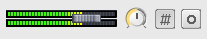 Playback in Sonic Visualiser is
controlled using the transport controls in the toolbar and the
fader/meter and playback speed controls in the bottom right of the
main window.
Playback in Sonic Visualiser is
controlled using the transport controls in the toolbar and the
fader/meter and playback speed controls in the bottom right of the
main window.
Use the ![]() Play / Pause button
to start and stop playback, and use
Play / Pause button
to start and stop playback, and use ![]() Rewind to Start and
Rewind to Start and ![]() Fast Forward to End to jump to either
end of the audio file.
Fast Forward to End to jump to either
end of the audio file.
The ![]() Rewind and
Rewind and ![]() Fast Forward buttons are
only active if the current layer is a time
instants or time value layer. If one of
these layers is current, these buttons will jump to the nearest item
in that layer.
Fast Forward buttons are
only active if the current layer is a time
instants or time value layer. If one of
these layers is current, these buttons will jump to the nearest item
in that layer.
You can also jump about during playback by simply dragging a pane
using the ![]() navigation tool,
provided the pane is set to follow playback.
navigation tool,
provided the pane is set to follow playback.
To be written:
-- play selection, loop (zero-crossing example)
-- volume, slowdown (and controls for them)
-- Layer playback (and controls for it – pan/volume/plugins)
-- Sample rates and resampling
The Application Preferences window (available through the Preferences option of the File menu) contains a number of things which may be adjusted to change the display or calculations carried out by Sonic Visualiser.
Press the keys 1 to 4 to change the current tool. Press 1 for ![]() the
navigate tool, 2 for
the
navigate tool, 2 for ![]() the select tool, 3 for
the select tool, 3 for ![]() the edit tool and 4 for
the edit tool and 4 for ![]() the draw tool.
the draw tool.
Press the keys 7, 8, 9, and 0 to change the text overlay display level.
Press 7 to display all available text overlays, including centre frame and time ruler markings, vertical scale information, and the names and stacking order of layers in the panes.
Press 8 to display basic textual information, omitting the layer names but retaining the vertical scale where appropriate.
Press 9 to display only time information, with no scale or textual overlays.
Press 0 to suppress all textual and timing information.
With the navigate tool ![]() selected, click and drag with the left or middle
mouse button in any pane to move the centre frame.
selected, click and drag with the left or middle
mouse button in any pane to move the centre frame.
When any other tool is selected, click and drag with the middle mouse button in any pane to move the centre frame.
Click and drag with any button in the navigation bar at the bottom of the window to move quickly around the audio file.
Press the Left and Right cursor keys to scroll the current pane by small increments. Press Ctrl and the Left and Right cursor keys to scroll in larger, half-window increments.
Roll the mouse wheel up, or press the Up cursor key, to zoom in; roll the wheel down or press the Down cursor key to zoom out.
Press Space to start or stop playback.
Press Page Up or Page Down to rewind or fast-forward to the next time instant or point in the active layer, if there is a time instants or time values layer active.
Press Home or End to rewind or fast-forward to either end of the file.
Press the keypad Enter key to insert a time instant at the current playback position, for real-time annotation. If the current layer is not a time instant layer, a new time instant layer will be created and added to the current pane and the new instant will be inserted into that.